Measure for Information, Not for Fitness: Designing Protein Experiments to Reveal Epistasis
A protein language model can rank thousands of mutations, but ranking is not the same as knowing which measurements to buy. This study spends a fixed experimental budget on the variants that expose how mutations interact. Registered downstream benchmarks back loop-count selection over fitness-greedy selection on GB1 and TrpB, while adding ESM masking dispersion buys no supported improvement.
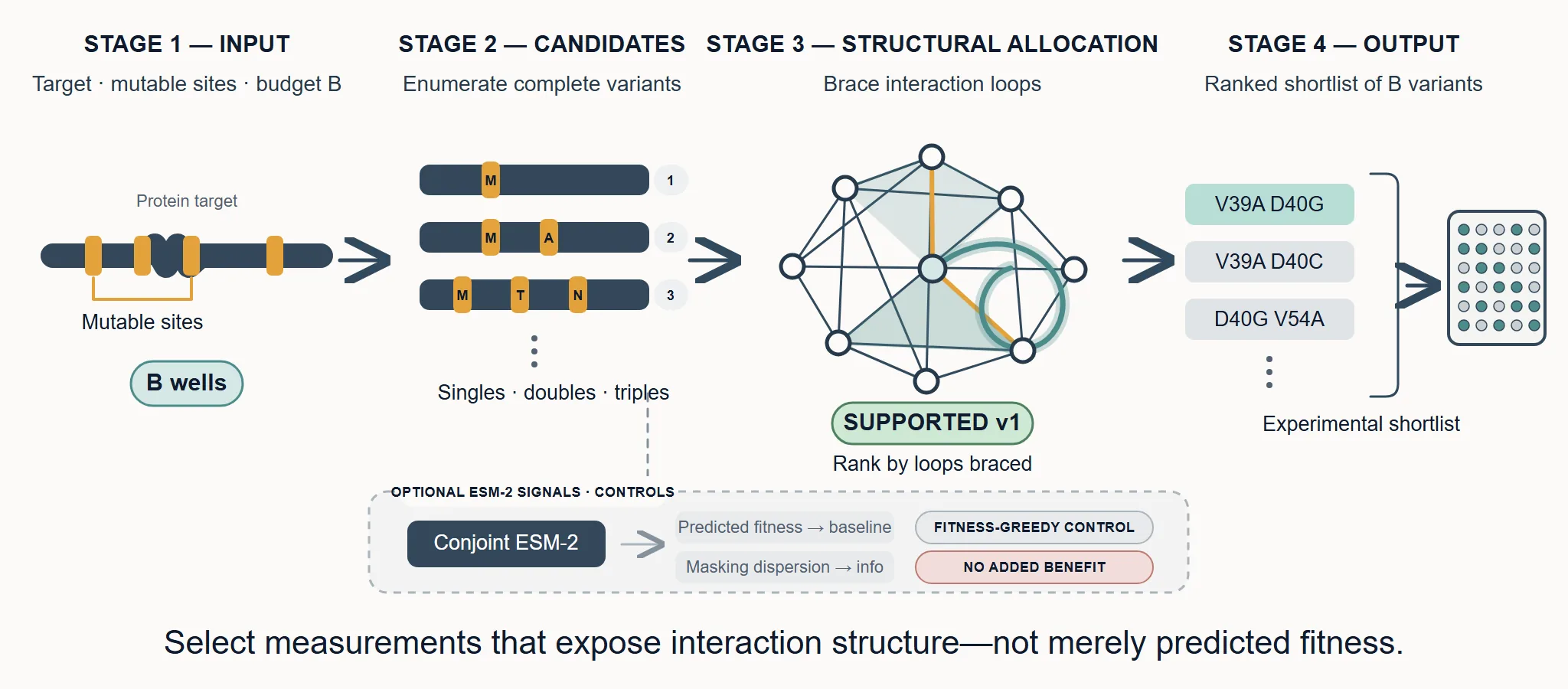
Figure n°1: From target protein to experimental plate
Description: epibudget scores complete variants, maps their interaction structure, and converts a fixed experimental budget into a ranked measurement plate.
A protein language model can score thousands of mutations before anyone touches a pipette. That suggests an obvious recipe for protein engineering: rank the variants, keep the top predictions, and test them.
The recipe answers one question. Which variants does the model expect to perform well? It stays silent on a second one. Which variants should we measure if we want to learn how mutations interact?
The two questions do not share an answer. A plate stacked with predicted winners is good for exploitation and often poor as data. When every well lands in the same small neighbourhood of sequence space, the experiment says little about why the landscape has its shape, or how an untested combination will behave.
I built epibudget to take the second question seriously. Given a fixed budget of wells, it selects variants meant to expose epistatic structure instead of simply maximizing predicted fitness.
The project started from a hypothesis about ESM masking dispersion. The finished evidence pulls that weighting term apart from loop coverage, and the two do not fare the same. On TrpB, info beats fitness and random for pairwise map recovery, while the loop-count baseline exceeds info at budgets 96 and 192. In the downstream benchmark, loop-count selection beats fitness-greedy in 20/20 partitions on both GB1 and TrpB. The masking-dispersion gate does not pass on either landscape.
Epistasis makes prediction a relational problem
Suppose mutation A shifts a protein's fitness by +0.2 and mutation B shifts it by +0.1. An additive model predicts +0.3 for the double mutant AB. If the measured effect is +0.8, the surplus +0.5 is pairwise epistasis:
A's effect now depends on whether B is present, and the reverse holds too. For three mutations, the same bookkeeping extends through inclusion–exclusion:
This is why a combination measured on its own is not enough. Pinning down an interaction also requires the surrounding members of its inclusion–exclusion loop. For a pair, that loop holds A, B, and AB relative to the reference protein. For a triple, it holds seven mutant measurements. Measure the whole family and the interaction is fixed. Leave members out and it has to be inferred.
So the candidate set is better read as a measurement network than as a bag of independent points, each carrying its own fitness score. Some variants sit inside many interaction loops. Measuring one of them braces several uncertain relationships at once.
Geodetic triangulation is the useful analogy. A survey network becomes informative when its measurements form constraints that have to close consistently. A protein experiment behaves the same way: its chosen singles, doubles, and triples become informative when they jointly constrain the epistasis map.
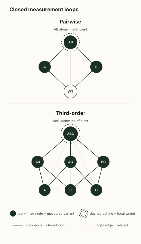
Figure n°2: Interaction coefficients are defined by closed measurement loops
Description: Pairwise and third-order coefficients are defined relative to WT-referenced families of measurements. An isolated combination cannot determine its own epistatic effect.
A plate budget changes the objective
The benchmarks use four mutable sites over the full 20-amino-acid alphabet. Restricting candidates to singles, doubles, and triples still leaves 29,678 variants: 76 singles, 2,166 doubles, and 27,436 triples.
The budgets are 48, 96, and 192 measurements. Even the largest simulated plate therefore covers less than one percent of that candidate universe.
Scarcity forces a choice. Spend those wells on the variants most likely to be fit? On a random sample? Or on variants that jointly constrain as many interactions as possible? Fitness-greedy selection is exploitation: it asks the model for its favourite sequences. Epistasis mapping is an information problem: it asks which measurements would make hidden interaction structure identifiable.
A two-part ESM-2 hypothesis
The registered profile used the 650-million-parameter checkpoint of ESM-2, a protein language model trained to reconstruct masked amino acids from their sequence context.
ESM-2 plays two roles. The first is to score every candidate without experimental labels, and it hides a technical trap. Score a double mutant by evaluating A and B independently on the original reference sequence and then summing, and the result is additive by construction. The model's pairwise epistasis collapses to exactly zero.
epibudget therefore scores variants conjointly. For AB, both mutations enter the sequence first. Position A is scored while B is present, position B while A is present, and the conditional log-likelihood ratios are then combined. Because each mutation is read in the other's context, the double-mutant score is free to differ from the sum of two reference-background single scores.
The second role is more speculative. For each candidate, random stretches of the surrounding, non-mutated sequence are masked and the same variant is rescored, 16 times in the registered profile. The variance across those scores becomes the masking-dispersion statistic. It measures how sensitive the score is to perturbed context, and it is not a calibrated posterior uncertainty estimate.
The intuition was defensible: prefer variants that matter to many interactions, then, among those, prefer the ones whose ESM score is most sensitive to context. It also bought a clean ablation. Assign every candidate the same dispersion and the weighting term vanishes, leaving the loop-count baseline (named structural in the tracked artifacts), which ranks variants only by how many pairwise and third-order loops they brace. The label points at interaction structure, not protein 3D structure.
This gives five strategies to compare: random sampling; fitness-greedy selection; a practice heuristic that starts from predicted beneficial singles and then adds their combinations; the low-order-first loop-count baseline; and the uncertainty-weighted score (named info in the tracked artifacts), which multiplies loop count by ESM masking dispersion.
Under the v1 independent-noise model, the acquisition score is modular: a candidate's score does not drop once a related candidate has already been selected. Allocation is therefore a fixed ranking, not a fully adaptive Bayesian design with correlated uncertainty and diminishing returns. That simplification made the first version tractable, and it marks the obvious next mathematical improvement.
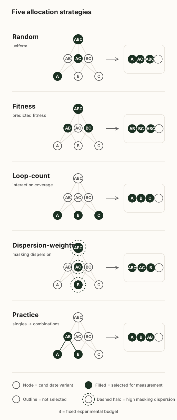
Figure n°3: Same candidates, different experimental plates
Description: Five static strategies select the same number of variants from a shared candidate universe. Only the selection criterion changes which variants enter the plate.
Evaluation without label leakage
The evaluation rests on two dense four-site landscapes. The first is GB1, an IgG-binding protein landscape introduced by Wu and colleagues. Its theoretical four-site space holds 20⁴, or 160,000, amino-acid combinations.
The second is TrpB, an enzyme active-site landscape from Johnston and colleagues. It offers a mechanistically different target (enzyme catalysis rather than protein binding), and the two landscapes are scored separately, never pooled into a single claim of generality.
The load-bearing validation rule is the label boundary. Candidate enumeration, ESM scoring, graph construction, and selection never read measured fitness. The plate is fixed first. Only then are the matching labels revealed from the public landscape, standing in for what a wet-lab run would return.
1. Map recovery
Once the selected measurements are revealed, the map-recovery benchmark reconstructs WT-referenced pairwise and third-order epistasis terms and compares them, by Pearson and Spearman correlation, against ground-truth terms computed from the dense measured landscape.
The benchmark asks whether the chosen plate helps recover the interaction map. It is not a measurements-only test: unmeasured loop members keep an ESM prior, so map recovery scores a measurement-plus-prior estimator.
2. Downstream prediction
The confirmatory downstream benchmark is more practical. Each selected plate trains the same fixed pairwise ridge model. That learner sees the revealed measurements, but no held-out ESM features and no prior-inclusive map-recovery output. It then ranks held-out double and triple mutants.
The registered primary score, Smacro, averages the Spearman correlations for doubles and triples. Every strategy faced the same learner, 20 partitions, five outer folds, and budgets of 48, 96, and 192. Loop-count selection beat fitness-greedy in 20/20 partitions on both landscapes, with a mean learning-curve AUC advantage of +0.342 on GB1 and +0.286 on TrpB.
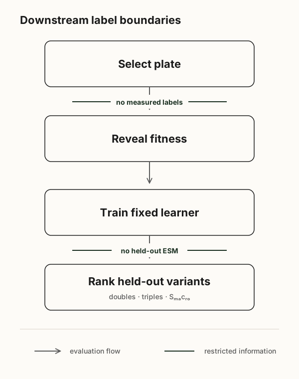
Figure n°4: Label boundaries in downstream evaluation
Description: Measured fitness is revealed only after selection, while held-out ESM features remain excluded from the fixed downstream learner.
What the V1 ablation actually compares
The historical V1 surrogate differs by a single weighting term. The loop-count baseline scores score(v) = n(v), where n(v) counts the interaction terms containing candidate v. The dispersion-weighted method scores score(v) = n(v) × τ²(v), where τ²(v) is the marginal dispersion of the ESM score across 16 masking perturbations.
Masking dispersion is an uncalibrated heuristic, not a validated posterior variance. The ablation therefore poses a deliberately narrow question: does that statistic add selection value on top of loop-count prioritization?
In the current symmetric four-site candidate universe, loop count is identical within each mutation order: 1,140 for singles, 39 for doubles, and 1 for triples. The baseline cannot discriminate inside an order, so historical rankings hinge on arbitrary tie-breaking or candidate enumeration order and call for a seeded tie reanalysis.
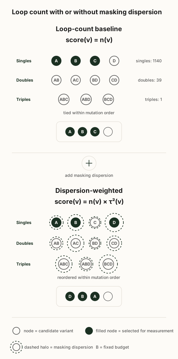
Figure n°5: What masking dispersion adds to the V1 score
Description: The ablation compares loop count alone with loop count weighted by ESM masking dispersion. Current evidence does not establish an additional benefit from the dispersion term.
Current evidence status
On TrpB, info beats fitness and random for pairwise map recovery. The loop-count baseline overtakes info at budgets 96 and 192, though not at 48. That pattern does not support a positive masking-dispersion contribution.
The corrective GB1 map-recovery result remains inconclusive_zero_gpu. Pairwise correlation improves at every registered budget, but relative squared-error gain stays negative, so no GB1 map-recovery winner is claimed.
The conforming downstream reports back loop-count selection over fitness-greedy in 20/20 partitions on GB1 and TrpB. They do not back the masking-dispersion contribution: the info-minus-loop-count gate passes in 15/20 GB1 partitions and 0/20 TrpB partitions at B = 192, below the registered threshold. Every comparative result remains provisional. The TrpB source mirror also carries 871 imputed fitness values that are not identified row by row.
What V1 established at the implementation level
- Variant selection can be posed as measurement design. Predicted fitness and expected experimental value are distinct objectives.
- Interaction-loop counts define a reproducible baseline. The implementation exposes exactly which interaction terms contain each candidate.
- Conjoint scoring preserves model epistasis. Applying every mutation before reading conditional scores avoids the additive shortcut that would erase interaction signal by construction.
- The masking-dispersion term can be isolated. The code supports a direct score-level ablation without dressing τ² up as calibrated uncertainty.
- The label-leakage barrier holds. The confirmatory benchmark fixes the plate before any measured fitness is available.
The completed downstream benchmark adds comparative evidence for the allocation objective: under the registered fixed learner, loop-count selection outperforms predicted-fitness selection on both landscapes. That does not establish generality beyond these datasets and this learner.
Why masking dispersion remains an open question
Sensitivity to a damaged sequence context is not the same as uncertainty about experimental error. A prediction can swing under artificial masking and still be accurate; it can also sit perfectly stable and be wrong. Current calibration evidence does not establish τ² as a posterior uncertainty estimate.
The V1 variance model also assumes errors are independent across variants. Members of an epistatic loop share sequence context and pass through the same model, so their errors may be correlated. Ignoring those covariances keeps the score simple but may drop information a meaningful information-gain calculation would need.
The conclusion stays narrow. Current provisional results do not support a positive masking-dispersion contribution. This is evidence about one static heuristic, two four-site landscapes, and one downstream learner; it is not evidence that contextual dispersion can never be useful.
Next validation steps
The current version is a single-shot allocator: it ranks the full candidate pool once and returns B variants. A stronger system would be sequential: measure a first plate, update a correlated posterior over variant effects and epistasis terms, then choose the next plate from what the experiment actually resolved.
That would make the geodetic analogy literal. Each new measurement would change the value of the ones still on the table. Redundant loops would show diminishing returns, while unresolved parts of the interaction graph would grow more valuable.
I would also keep three quantities apart that the first version partly ran together: a variant's predicted effect; its calibrated predictive error; and the experimental value of measuring it inside a network. The first helps predict. The second describes confidence. The third depends on the scientific question and on what has already been measured. One score should not stand in for all three.
Implications for experimental design
Protein language models make predictions cheap. Experiments stay scarce. That asymmetry is what makes allocation matter more over time: as candidate generation scales, the bottleneck moves from proposing sequences to deciding which evidence is worth buying.
epibudget did not validate its original masking-dispersion hypothesis. It did produce a comparative result for the simpler design principle: covering interaction loops built better downstream training plates than fitness-greedy selection on GB1 and TrpB under the registered learner. The result is provisional and does not establish broader generality.
The useful question is not “Which variants does the model like?” but “Which measurements make the interaction structure identifiable?” That is the criterion that should shape the next experimental round.
Evidence and sources
- Lin, Z. et al. Evolutionary-scale prediction of atomic-level protein structure with a language model. Science (2023).
- Wu, N. C. et al. Adaptation in protein fitness landscapes is facilitated by indirect paths. eLife (2016).
- Johnston, K. E. et al. A combinatorially complete epistatic fitness landscape in an enzyme active site. PNAS (2024).
- Frozen validation protocol, limitations, and tracked evidence artifact.